Controls System Commands

Let us analyze longitudinal dynamics representative of a transport aircraft, trimmed at $V_0 = 250$ ft/s and flying at a low altitude. The example is taken from 'Robust and Adaptive Control: With Aerospace Applications' by Eugene Lavretsky and Kevin Wise.

The linearized dynamics are given by the matrix $$ A = \begin{pmatrix} -0.038 & 18.984 & 0 & -32.174 \\ -0.001 & -0.632 & 1 & 0 \\ 0 & -0.759 & -0.518 & 0 \\ 0 & 0 & 1 & 0 \end{pmatrix} $$ To enter this matrix in CCST type matrix A '[[-0.038, 18.984, 0, -32.174], [-0.001,-0.632, 1, 0], [0, -0.759, -0.518, 0], [0, 0, 1, 0]]'

We can enter gdisplay A to view the entered matrix in latex rendering under the terminal. In turn, display A will display A in the console.

To calculate eigenvectors and eigenvalues of A enter the command modes A V E , where the last two arguments specify the variables were the results will be stored.

Next, let us define a matrix $B$ with control derivatives as follows: matrix B '[[10.1, 0], [0, -0.0086], [0.025, -0.011], [0,0]]'

Finally we will define two more matrices, $C$ and $D$ to complete our state space system with state feedback.

matrix C '[[1, 0, 0, 0], [0, 1, 0, 0], [0, 0, 1, 0], [0, 0, 0, 1]]'

matrix D '[[0, 0], [0, 0], [0, 0], [0, 0]]'

Next, we define the state system with the command ss A B C D G. The last argument gives the name of the state system. We can now graphically display the system with gdisplay G

Before connecting a feedback controller, let us simulate the angle of attack response to a step elevator command. We first let the system know that the elevator is the second input and the angle of attack is the second output with commands:

control 2 G elevator

output 2 G alpha

Now we can simulate the response to a 0.5 radian elevator deflection for 5 seconds with: step alpha G elevator 0.5 5 alpha_plot and view the result with gdisplay alpha_plot.

For a closed-loop system we define a controller in a standard space-state form with the command:

controller A B1 B2 C D1 D2 K

and arrange $G$ and $K$ into a feedback loop with:

feedback G K G_cl

Here, again the last argument gives a name to the resulting closed loop system.

To obtain response to initial conditions we can use the command:

response alpha G '[[0],[0]]' '[[0]]', 5.0 closed_loop_plot

Here the second argument specifies the initial conditions and the third argument specifies the reference input.

Path Planning Toolbox

For speed the toolbox uses Python code for some of the functionality and C++ code for other.

Local Planner and 2D Car Dynamics

Algorithms like Dijkstra's or RDT/RRT are often very useful as global path planners, however there are situations when dynamic constraints have to be taken into account. There are several ways to model these dynamics. One could describe the car with the following state variables: the position of its center of mass in the Cartesian coordinates, $x$, $y$, its angle of orientation, $\xi$, its velocity, $v$, and its mass, $m$. The inputs that can be controlled will be the amount of thrust applied, $\delta T$, the amount of breaking, $\delta B$, and the angle by which the front wheels are turned, $\delta w$. Below is a diagram summarizing this variables.

The next step is to derive a differential equation that describes the dynamics. The velocity components in the $x$ and $y$ directions can be simply obtained as vector projections of $v$ onto the coordinate axis using trigonometry, $$ \dot{x} = v \cos(\xi), $$ $$ \dot{y} = v \sin(\xi). $$ We'll also assume that the mass changes as a function of velocity and the throttle, i.e. $$ \dot{m} = g(v, \delta T). $$ This can be specified more explicitly depending on the properties of the actual car.

Next we use Newton's Second law, $F = m a = m \dot{v}$, written in terms of the velocity $v$.  To keep things a bit general we will assume that the total thrust provided by the car is $T(v, \delta T, \delta B)$, a function of the current velocity, as well as throttle and break amount. We also assume that the component of $T$ perpendicular to the tire has an equal friction force in the opposite direction to cancel it, leaving the parallel component, $T \cos(\delta w)$ as the net force (see the picture for the force diagram).  In turn, this force has components $T \cos(\delta w) \cos(\delta w)$ in the direction of forward acceleration, $\dot{v}$ and $T \cos(\delta w) \sin(\delta w)$ in the tangential direction.  It follows that, $$ m \dot{v} = T \cos^2 (\delta w) - D(v), $$ where the last term is the drag due to air resistance, often approximated with, $C_D \rho v^2 S/2$, where $C_D$ is the drag coefficient, $\rho$ is the density of air, $S$ is the area of the surface.  We'll keep this as $D(v)$ to keep things general.

The effect of the tangential force $T \cos(\delta w) \sin(\delta w)$ is slightly more technical to derive using Newton's Law. To keep things relatively simple, we'll use a slightly different argument to obtain an expression for the angular velocity $\dot{\xi}$. Assume that in time $\Delta t$ the base of the car moved $v \Delta t$ in original direction, $\xi$, while the orientation $\xi$ changed by $\Delta \xi$ as shown in the zoomed in picture below

Then, using the law of sines from trigonometry yields $$ \frac{l}{\sin(180-\delta w)} = \frac{l - v \Delta t}{\sin(\delta w - \Delta \xi)}, $$ or after simplification \begin{equation} \label{m2} l \sin(\delta w - \Delta \xi) = l \sin(\delta w) - v \Delta t \sin(\delta w). \end{equation} Note that by the mean value theorem $\sin(\delta w) - \sin(\delta w - \Delta \xi) = \cos(\delta w_*) \Delta \xi$ for some value of $\delta w_*$ between $\delta w - \Delta \xi$ and $\delta w$. Substituting the expression for $\sin(\delta w - \Delta \xi) $ into \eqref{m2} results in, $$ l \sin(\delta w) - l \Delta \xi \cos(\delta w_*) = l \sin(\delta w) - v \Delta t \sin(\delta w), $$ or after simplification $$ \frac{\Delta \xi}{\Delta t} = \frac{v}{l} \frac{\sin(\delta w)}{\cos(\delta w_*)} $$ Finally, taking the limit as $\Delta t \rightarrow 0$ (and consequently $\delta w_* \rightarrow \delta w$), we have $$ \frac{d \xi}{ dt} = \frac{v}{l} \tan(\delta w). $$

Minimum Jerk Trajectories

To calculate a 5 second minimum jerk lane-change trajectory that takes a car traveling at 5m/s to the lane 4 meters to the left at the position 20 meters ahead we can run:

generate_2d_traj '[-20, 0]' '[5, 0]' '[0, 0]' '[0, 4]' '[5, 0]' '[0, 0]' 5 lane_plot

Here the arguments specify initial position $[x,y]$, initial velocity $[v_x, v_y]$, initial acceleration $[a_x, a_y]$, final position, final velocity, final accelereration, and the time to perform the maneuver.

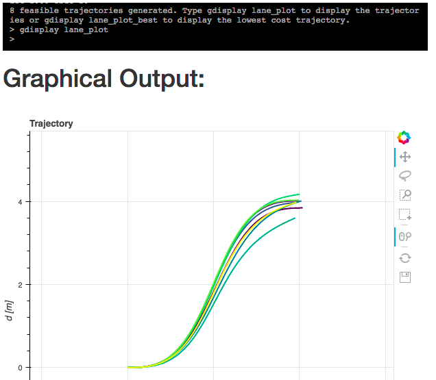
In real world trajectory generation oftentimes it is not enough to simply generate one optimal trajectory. In practice, one way to approach motion planning for lane changes or turns is to generate many possible trajectories by varying the final conditions and then selecting the best trajectory based on a more complicated cost function that could include, for example, distance to collisions, distance to the center of the lane, fuel consumption, etc. Running the command

generate_2d_traj '[-20, 0]' '[5, 0]' '[0, 0]' '[0, 4]' '[5, 0]' '[0, 0]' 5 lane_plot 1000 True 20

generates 20 trajectories by varying the final velocities and positions, and chooses the best path based on ensuring forward direction of motion and jerk minimization. The additional parameters above specify number of grid points (1000), a flag that specifies that many trajectories should be sampled (True), and the number of trajectories to sample.

A sample result is shown below:

My implementation of these solvers can be found here: C++ Code

The bvp solver is generic enough to handle not just the Euler-Lagrange equations corresponding to jerk minimization, but analogous functionals with arbitrary high derivatives and arbitrary number of waypoints.

For a more general collocation based bvp solver see: C++ Code

Coming soon: $H^\infty$ Control for Trajectory Tracking

Optimal Stopping Control

To calculate the optimal control history to bring a car traveling at 20 m/s to a complete stop in 500 m we can run

generate_optimal_stop_traj 20 500 stop_plot

Dijkstra's Algorithm

One way to use Dijkstra's algorithm is to represent the map as a grid using an $m$ by $n$ matrix. To avoid entering a large matrix by hand the toolbox allows to upload any image whose grayscale can be thresholded to produce the obstacles. As an example consider the image below:

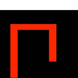
To upload the image expand the menu at the top right corner, above the console screen. Give a name to this image, for example `map1`. This will be the handle for working with the image from the console.

After uploading the file we can display the uploaded image with gdisplay map1. To generate a grid by thresholding grayscale values of the image we can use generate_grid map1 15 15 where map1 is the handle of the uploaded image and the last two parameters specify the height and width of the grid. The matrix representing the grid will be saved under map1_grid name with values at each cell representing the grayscale value of the image.

Entering gdisplay map1_grid displays this matrix. To turn these values into free space and obstacle regions needed to run Dijkstra's algorithm we can enter:

generate_grid_obstacles map1_grid 2 map2_grid

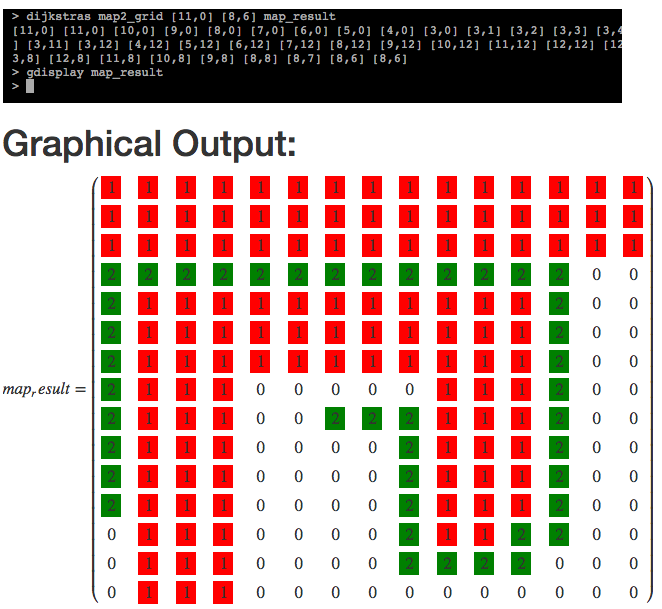
This sets cells with value larger than 2 to 1 (representing obstacle region) and cells with values less than or equal to 2 to 0 (representing free space). We can display the resulting matrix with:

gdisplay map2_grid

Finally, running dijkstras map2_grid [11,0] [8,6] map_result finds a path from the (11,0) position on the grid to the (8,6) position.

Orbital Mechanics Toolbox

The toolbox uses C++ code under the hood.

Lambert's Problem

Consider a satellite to be located at $r_1 = 5000 \hat{I} + 10000 \hat{J} + 2100 \hat{K}$ km. We want to design a trajectory that will put the satellite at $r_2 = -14600 \hat{I} + 2500 \hat{J} + 7000 \hat{K}$ km after one hour. This is achieved by solving Lambert's problem, by calling

lambert '[5000, 10000, 2100]' '[-14600, 2500, 7000]' 3600 True 398600 orbit1

Here we specified the two positions, time, whether we want the prograde trajectory, $\mu$, and a name to save the results under. To see the orbital elements associated with the calculated orbit we simply type:

gdisplay orbit1

Optimal Circular Orbit Transfer

Consider establishing the optimal transfer trajectory to get from a given circular orbit around the earth to the largest radial position in a given amount of time using constant thrust and the thrust angle as the control. This problem can be posed as a classic optimal control problem of finding extrema of a functional of the form $$ J(\alpha) := \int_{t_0}^{t_f} L(t,x(t),\alpha(t)) \, dt + K(t_f, x_f), $$ $$ \dot{x} = f(t, x, \alpha), \quad x(t_0) = x_0, $$ where the running cost $L \equiv 0$ and the terminal cost $K := r(t_f)$ is the final radial position. Precisely,

$$ J = r(t_f), $$ subject to the classic two-body equations of motion in polar coordinates $$ \begin{align} \dot{r} & = u, \\ \dot{u} & = \frac{v^2}{r} - \frac{\mu}{r^2} + \frac{T \sin \alpha}{m_0 - |\dot{m}|t}, \\ \dot{v} & = -\frac{u v}{r} + \frac{T \cos\alpha}{m_0 - |\dot{m} t|}, \\ \dot{\theta} & = \frac{v}{r}, \end{align} $$

where $r$ is the radial position of the vehicle, $u$ and $v$ are radial and tangential velocities, $T$ is the thrust applied at the angle of $\alpha$ radians. In addition, $m_0$ is the initial vehicle mass and $\dot{m}$ is the mass flow rate. (See James M Longuski, José J. Guzmán, John E. Prussing, Optimal Control with Aerospace Applications-Springer-Verlag New York (2014))

By the use of Pontryagin's Maximum Principle, this problem can be reduced to solving a boundary value problem $$ \begin{align} \frac{d \bar{r}}{d \tau} & = \bar{u} \eta, \\ \frac{d \bar{u}}{d \tau} & = \left( \frac{\bar{v}^2}{\bar{r} - \frac{1}{\bar{r}^2}} \right) \eta + \frac{\bar{T}}{m_0 - |\dot{m}| \tau t_f} \left( \frac{p_u}{\sqrt{p_u^2+p_{v}^2}} \right), \\ \frac{d \bar{v}}{d \tau} & = \frac{\bar{u}{\bar{v}}{\bar{r}}}\eta + \frac{\bar{T}}{m_0 - |\dot{m}| \tau t_f} \left( \frac{p_{v}}{\sqrt{p_u^2+p_{v}^2}} \right), \\ \frac{d \theta}{d \tau} & = \frac{\bar{v}{\bar{r}}} \eta, \\ \frac{d p_r}{d \tau} & = p_u \left(\frac{\bar{v}^2}{\bar{r}^2} -\frac{2}{\bar{r}^3} \right) \eta - p_{v} \frac{\bar{u}{\bar{v}}}{\bar{r}^2} \eta + \frac{p_{\theta} \bar{v}}{\bar{r}^2} \eta, \\ \frac{d p_u}{d \tau} & = -p_r \eta + \frac{p_{v} \bar{v}}{\bar{r}}, \\ \frac{d p_v}{d \tau} & = -\frac{2 p_u v \eta}{\bar{r}} + \frac{p_{v} u \eta}{\bar{r}} - {p_{\theta} \eta}{\bar{r}}, \end{align} $$ for the rescaled variables $$ \bar{r} = \frac{r}{r(0)}, \, \bar{u} = \frac{u}{v(0)}, \, \bar{v} = \frac{v}{v(0)}, \, \tau = \frac{t}{t_f}, $$ the co-states $p_r, p_{\theta}, p_u, p_v$ and subject to the boundary conditions $$ \begin{cases} \bar{r}_0(0) = 1, \, \bar{u}(0) = 0, \, \bar{v}(0)=1, \, \theta(0) = 0, \\ \bar{u}(1) = 0, \, \bar{v}(1) = \sqrt{1/\bar{r}(1)}, \, 1 - p_r(1) + \frac{1}{2} p_v(1) \sqrt{1/\bar{r}^3(1)} = 0, \, p_{\theta}(1) = 0 \end{cases} $$ To solve the problem with $\mu = 3.986004418e5$, initial mass $m_0 = 1500$ kg, specific impulse $I_{sp} = 6000$, thrust $T = 20$ N, initial orbit radius $6678$ km, final time $t_f = 0.5$ days, and using 5 hour timesteps and 500 grid points for each timestep we run

orb_transfer_lobatto3 3.986004418e5 1500 6000 20 6678 0.5 5 500 traj_plot

The above solves the problem using a three stage Lobatto collocation scheme: $$ \begin{array}{c|ccc} 0 & 0 & 0 & 0 \\ 1/2 & 5/24 & 1/3 & -1/24 \\ 1 & 1/6 & 2/3 & 1/6 \\ \hline & 1/6 & 2/3 & 1/6 \end{array} $$ Similarly, we can run a generic collocation code by specifying the scheme at the end of the command. For example, to use a trapezoid scheme, $$ \begin{array}{c|cc} 0 & 0 & 0 \\ 1 & 1/2 & 1/2 \\ \hline & 1/2 & 1/2 \end{array} $$ we can enter

orb_transfer 3.986004418e5 1500 6000 20 6678 0.5 5 500 2 [0,1] [[0,0],[0.5,0.5]] [0.5,0.5] traj_plot

My implementation of this boundary value problem solver can be found here: C++ Code

The resulting plots can be displayed with

gdisplay traj_plot and gdisplay traj_plot_control

Collocation Method

We consider a system of differential equations of the form $$ y' = f(t,y) $$ $$ g(y(a), y(b)) = 0$$ For fixed $t$ and $y$, let $A = \frac{\partial f}{\partial y}(t,y)$, $B_1 = \partial_1 g$, $B_2 = \partial_2 g$

Uploading an Image

The first step is to upload an image to be analyzed. To do that expand the menu at the top right corner, above the console screen and upload an image. Give a name to this image, for example `image1`. This will be the handle for working with the image from the console.

After uploading the file we can display the uploaded image with gdisplay image1.

Comning soon: semantic segmentation instructions.